Getting Started with ctapipe

This hands-on was presented at the Paris CTAO Consoritum meeting (K. Kosack)

Part 1: load and loop over data

import glob

import numpy as np
import pandas as pd
from ipywidgets import interact
from matplotlib import pyplot as plt

from ctapipe import utils
from ctapipe.calib import CameraCalibrator
from ctapipe.image import hillas_parameters, tailcuts_clean
from ctapipe.io import EventSource, HDF5TableWriter
from ctapipe.visualization import CameraDisplay

# %matplotlib inline

path = utils.get_dataset_path("gamma_prod5.simtel.zst")

source = EventSource(path, max_events=5)

for event in source:
    print(event.count, event.index.event_id, event.simulation.shower.energy)

0 4009 0.07287972420454025 TeV
1 5101 1.7454713582992554 TeV
2 5103 1.7454713582992554 TeV
3 5104 1.7454713582992554 TeV
4 5105 1.7454713582992554 TeV

event

ctapipe.containers.ArrayEventContainer:
                       index.*: event indexing information with default None
                          r0.*: Raw Data with default None
                          r1.*: R1 Calibrated Data with default None
                         dl0.*: DL0 Data Volume Reduced Data with default None
                         dl1.*: DL1 Calibrated image with default None
                         dl2.*: DL2 reconstruction info with default None
                  simulation.*: Simulated Event Information with default None
                                with type <class
                                'ctapipe.containers.SimulatedEventContainer'>
                     trigger.*: central trigger information with default None
                         count: number of events processed with default 0
                  monitoring.*: container for event-wise monitoring data (MON)
                                with default None
                        muon.*: Container for muon analysis results with default
                                None

event.r1

ctapipe.containers.R1Container:
                        tel[*]: map of tel_id to R1CameraContainer with default
                                None

for event in EventSource(path, max_events=5):
    print(event.count, event.r1.tel.keys())

0 dict_keys([9, 14, 104])
1 dict_keys([26, 27, 29, 47, 53, 59, 69, 73, 121, 122, 124, 148, 162, 166])
2 dict_keys([82, 92, 175, 179])
3 dict_keys([17, 26, 27, 29, 43, 47, 53, 57, 69, 112, 121, 122, 124, 125, 128, 140, 144, 148, 162, 166])
4 dict_keys([3, 4, 8, 9, 14, 15, 23, 24, 25, 29, 32, 36, 42, 46, 52, 56, 103, 104, 109, 110, 118, 119, 120, 126, 127, 129, 130, 137, 139, 143, 161])

event.r0.tel[3]

ctapipe.containers.R0CameraContainer:
                      waveform: numpy array containing ADC samples: (n_channels,
                                n_pixels, n_samples) with default None

r0tel = event.r0.tel[3]

r0tel.waveform

array([[[432, 413, 395, ..., 382, 387, 382],
        [419, 420, 428, ..., 392, 396, 405],
        [381, 392, 413, ..., 375, 387, 387],
        ...,
        [391, 384, 385, ..., 379, 395, 404],
        [370, 376, 388, ..., 391, 383, 383],
        [393, 411, 413, ..., 406, 392, 396]],

       [[413, 396, 398, ..., 397, 401, 395],
        [392, 407, 403, ..., 403, 388, 399],
        [405, 403, 393, ..., 393, 400, 409],
        ...,
        [399, 406, 407, ..., 391, 405, 397],
        [401, 399, 396, ..., 395, 400, 388],
        [399, 393, 403, ..., 395, 407, 401]]],
      shape=(2, 1855, 40), dtype=uint16)

r0tel.waveform.shape

(2, 1855, 40)

note that this is (\(N_{channels}\), \(N_{pixels}\), \(N_{samples}\))

plt.pcolormesh(r0tel.waveform[0])

<matplotlib.collections.QuadMesh object at 0x79f092887190>

brightest_pixel = np.argmax(r0tel.waveform[0].sum(axis=1))
print(f"pixel {brightest_pixel} has sum {r0tel.waveform[0,1535].sum()}")

pixel 1831 has sum 15824

plt.plot(r0tel.waveform[0, brightest_pixel], label="channel 0 (high-gain)")
plt.plot(r0tel.waveform[1, brightest_pixel], label="channel 1 (low-gain)")
plt.legend()

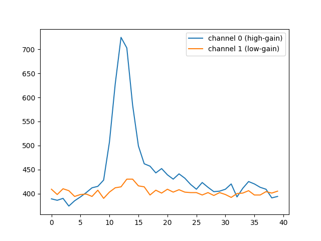
<matplotlib.legend.Legend object at 0x79f094b006a0>

@interact
def view_waveform(chan=0, pix_id=brightest_pixel):
    plt.plot(r0tel.waveform[chan, pix_id])

interactive(children=(IntSlider(value=0, description='chan', max=1), IntSlider(value=1831, description='pix_id', max=5493, min=-1831), Output()), _dom_classes=('widget-interact',))

try making this compare 2 waveforms

Part 2: Explore the instrument description

This is all well and good, but we don’t really know what camera or telescope this is… how do we get instrumental description info?

Currently this is returned inside the event (it will soon change to be separate in next version or so)

subarray = source.subarray

subarray

SubarrayDescription(name='MonteCarloArray', n_tels=180)

subarray.peek()

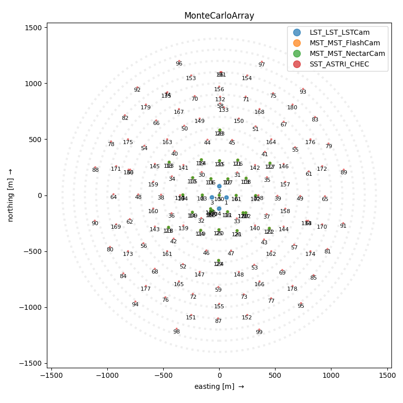
<ctapipe.visualization.mpl_array.ArrayDisplay object at 0x79f091b47340>

subarray.to_table()

Table length=180

tel_id	name	type	pos_x	pos_y	pos_z	camera_name	optics_name	camera_index	optics_index	tel_description
			m	m	m
uint16	str5	str3	float32	float32	float32	str9	str5	int64	int64	str17
1	LST	LST	-20.643	-64.817	34.3	LSTCam	LST	2	1	LST_LST_LSTCam
2	LST	LST	79.993996	-0.768	29.4	LSTCam	LST	2	1	LST_LST_LSTCam
3	LST	LST	-19.396	65.2	31.0	LSTCam	LST	2	1	LST_LST_LSTCam
4	LST	LST	-120.033	1.151	33.1	LSTCam	LST	2	1	LST_LST_LSTCam
5	MST	MST	-0.017	-0.001	24.35	FlashCam	MST	1	2	MST_MST_FlashCam
6	MST	MST	-1.468	-151.221	31.0	FlashCam	MST	1	2	MST_MST_FlashCam
7	MST	MST	-3.1379998	-325.245	39.0	FlashCam	MST	1	2	MST_MST_FlashCam
8	MST	MST	1.4339999	151.22	25.0	FlashCam	MST	1	2	MST_MST_FlashCam
9	MST	MST	3.1039999	325.243	23.5	FlashCam	MST	1	2	MST_MST_FlashCam
...	...	...	...	...	...	...	...	...	...	...
172	ASTRI	SST	260.0	-920.0	65.0	CHEC	ASTRI	0	0	SST_ASTRI_CHEC
173	ASTRI	SST	-500.0	815.0	15.0	CHEC	ASTRI	0	0	SST_ASTRI_CHEC
174	ASTRI	SST	-500.0	-815.0	75.0	CHEC	ASTRI	0	0	SST_ASTRI_CHEC
175	ASTRI	SST	500.0	815.0	45.0	CHEC	ASTRI	0	0	SST_ASTRI_CHEC
176	ASTRI	SST	500.0	-815.0	53.0	CHEC	ASTRI	0	0	SST_ASTRI_CHEC
177	ASTRI	SST	-810.0	655.0	12.0	CHEC	ASTRI	0	0	SST_ASTRI_CHEC
178	ASTRI	SST	-810.0	-655.0	68.0	CHEC	ASTRI	0	0	SST_ASTRI_CHEC
179	ASTRI	SST	810.0	655.0	20.0	CHEC	ASTRI	0	0	SST_ASTRI_CHEC
180	ASTRI	SST	810.0	-655.0	41.0	CHEC	ASTRI	0	0	SST_ASTRI_CHEC

subarray.tel[2]

TelescopeDescription(type='LST', optics_name='LST', camera_name='LSTCam')

subarray.tel[2].camera

CameraDescription(name=LSTCam, geometry=LSTCam, readout=LSTCam)

subarray.tel[2].optics

OpticsDescription(name=LST, size_type=LST, reflector_shape=PARABOLIC, equivalent_focal_length=28.00 m, effective_focal_length=29.31 m, n_mirrors=1, mirror_area=386.73 m2)

tel = subarray.tel[2]

tel.camera

CameraDescription(name=LSTCam, geometry=LSTCam, readout=LSTCam)

tel.optics

OpticsDescription(name=LST, size_type=LST, reflector_shape=PARABOLIC, equivalent_focal_length=28.00 m, effective_focal_length=29.31 m, n_mirrors=1, mirror_area=386.73 m2)

tel.camera.geometry.pix_x

<Quantity [ 0.        , -0.0377967 , -0.04724547, ...,  0.67088033,
           -0.45356484, -0.50081024] m>

tel.camera.geometry.to_table()

Table length=1855

pix_id	pix_x	pix_y	pix_area
	m	m	m2
int64	float64	float64	float64
0	0.0	0.0	0.002079326892271638
1	-0.037796701200384926	-0.032732429036768325	0.002079326892271638
2	-0.04724547496329345	0.01636666208397624	0.002079326892271638
3	-0.009448773762908523	0.049099091120744565	0.002079326892271638
4	0.037796701200384926	0.032732429036768325	0.002079326892271638
5	0.04724547496329345	-0.01636666208397624	0.002079326892271638
6	0.009448773762908523	-0.049099091120744565	0.002079326892271638
7	-0.07559330728842001	-0.0654648397698358	0.002079326892271638
8	-0.08504208105132853	-0.016365748649091242	0.002079326892271638
...	...	...	...
1846	-0.6708803327659516	0.9656188254531993	0.002079326892271638
1847	0.45356483600883174	1.0801754621151205	0.002079326892271638
1848	0.50081024449667	1.063808751198785	0.002079326892271638
1849	1.1622417344092089	0.14728906047502396	0.002079326892271638
1850	1.1716905074681288	0.09818997301244671	0.002079326892271638
1851	0.708676884320607	-0.9328863284767506	0.002079326892271638
1852	0.6708803327659516	-0.9656188254531993	0.002079326892271638
1853	-0.45356483600883174	-1.0801754621151205	0.002079326892271638
1854	-0.50081024449667	-1.063808751198785	0.002079326892271638

tel.optics.mirror_area

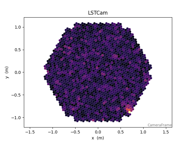
<Quantity 386.73324585 m2>

disp = CameraDisplay(tel.camera.geometry)

disp = CameraDisplay(tel.camera.geometry)
disp.image = r0tel.waveform[
    0, :, 10
]  # display channel 0, sample 0 (try others like 10)

** aside: ** show demo using a CameraDisplay in interactive mode in ipython rather than notebook

Part 3: Apply some calibration and trace integration

calib = CameraCalibrator(subarray=subarray)

for event in EventSource(path, max_events=5):
    calib(event)  # fills in r1, dl0, and dl1
    print(event.dl1.tel.keys())

dict_keys([9, 14, 104])
dict_keys([26, 27, 29, 47, 53, 59, 69, 73, 121, 122, 124, 148, 162, 166])
dict_keys([82, 92, 175, 179])
dict_keys([17, 26, 27, 29, 43, 47, 53, 57, 69, 112, 121, 122, 124, 125, 128, 140, 144, 148, 162, 166])
dict_keys([3, 4, 8, 9, 14, 15, 23, 24, 25, 29, 32, 36, 42, 46, 52, 56, 103, 104, 109, 110, 118, 119, 120, 126, 127, 129, 130, 137, 139, 143, 161])

event.dl1.tel[3]

ctapipe.containers.DL1CameraContainer:
                         image: Numpy array of camera image, after waveform
                                extraction.Shape: (n_pixel) if n_channels is 1
                                or data is gain selectedelse: (n_channels,
                                n_pixel) with default None
                     peak_time: Numpy array containing position of the peak of
                                the pulse as determined by the extractor.Shape:
                                (n_pixel) if n_channels is 1 or data is gain
                                selectedelse: (n_channels, n_pixel) with default
                                None
                    image_mask: Boolean numpy array where True means the pixel
                                has passed cleaning. Shape: (n_pixel, ) with
                                default None as a 1-D array with dtype bool
                      is_valid: True if image extraction succeeded, False if
                                failed or in the case of TwoPass methods, that
                                the first pass only was returned. with default
                                False
                    parameters: Image parameters with default None with type
                                <class
                                'ctapipe.containers.ImageParametersContainer'>

dl1tel = event.dl1.tel[3]

dl1tel.image.shape  # note this will be gain-selected in next version, so will be just 1D array of 1855

(1855,)

dl1tel.peak_time

array([27.381046, 17.746258, 18.80205 , ..., 11.64868 , 31.961287,
       29.717525], shape=(1855,), dtype=float32)

CameraDisplay(tel.camera.geometry, image=dl1tel.image)

<ctapipe.visualization.mpl_camera.CameraDisplay object at 0x79f097085930>

CameraDisplay(tel.camera.geometry, image=dl1tel.peak_time)

<ctapipe.visualization.mpl_camera.CameraDisplay object at 0x79f094b58d00>

Now for Hillas Parameters

image = dl1tel.image
mask = tailcuts_clean(tel.camera.geometry, image, picture_thresh=10, boundary_thresh=5)
mask

array([False, False, False, ..., False, False, False], shape=(1855,))

CameraDisplay(tel.camera.geometry, image=mask)

<ctapipe.visualization.mpl_camera.CameraDisplay object at 0x79f091770910>

cleaned = image.copy()
cleaned[~mask] = 0

disp = CameraDisplay(tel.camera.geometry, image=cleaned)
disp.cmap = plt.cm.coolwarm
disp.add_colorbar()
plt.xlim(0.5, 1.0)
plt.ylim(-1.0, 0.0)

(-1.0, 0.0)

params = hillas_parameters(tel.camera.geometry, cleaned)
print(params)

{'intensity': np.float64(32.78351974487305),
 'kurtosis': np.float64(1.2333006676347782),
 'length': <Quantity 0.02219065 m>,
 'length_uncertainty': <Quantity 0.00093599 m>,
 'phi': <Angle -0.88747705 rad>,
 'psi': <Angle -1.56935711 rad>,
 'psi_uncertainty': <Angle 2.08329213 rad>,
 'r': <Quantity 1.11337613 m>,
 'skewness': np.float64(-0.271615381552047),
 'transverse_cog_uncertainty': <Quantity 0.00796404 m>,
 'width': <Quantity 0.01614423 m>,
 'width_uncertainty': <Quantity 0.00226475 m>,
 'x': <Quantity 0.70295289 m>,
 'y': <Quantity -0.86340237 m>}

disp = CameraDisplay(tel.camera.geometry, image=cleaned)
disp.cmap = plt.cm.coolwarm
disp.add_colorbar()
plt.xlim(0.5, 1.0)
plt.ylim(-1.0, 0.0)
disp.overlay_moments(params, color="white", lw=2)

Ignoring fixed x limits to fulfill fixed data aspect with adjustable data limits.

Part 4: Let’s put it all together:

• loop over events, selecting only telescopes of the same type (e.g. LST:LSTCam)

• for each event, apply calibration/trace integration

• calculate Hillas parameters

• write out all hillas parameters to a file that can be loaded with Pandas

first let’s select only those telescopes with LST:LSTCam

subarray.telescope_types

(TelescopeDescription(type='SST', optics_name='ASTRI', camera_name='CHEC'), TelescopeDescription(type='LST', optics_name='LST', camera_name='LSTCam'), TelescopeDescription(type='MST', optics_name='MST', camera_name='NectarCam'), TelescopeDescription(type='MST', optics_name='MST', camera_name='FlashCam'))

subarray.get_tel_ids_for_type("LST_LST_LSTCam")

(1, 2, 3, 4)

Now let’s write out program

data = utils.get_dataset_path("gamma_prod5.simtel.zst")
source = EventSource(data)  # remove the max_events limit to get more stats

for event in source:
    calib(event)

    for tel_id, tel_data in event.dl1.tel.items():
        tel = source.subarray.tel[tel_id]
        mask = tailcuts_clean(tel.camera.geometry, tel_data.image)
        if np.count_nonzero(mask) > 0:
            params = hillas_parameters(tel.camera.geometry[mask], tel_data.image[mask])

with HDF5TableWriter(filename="hillas.h5", group_name="dl1", overwrite=True) as writer:
    source = EventSource(data, allowed_tels=[1, 2, 3, 4], max_events=10)
    for event in source:
        calib(event)

        for tel_id, tel_data in event.dl1.tel.items():
            tel = source.subarray.tel[tel_id]
            mask = tailcuts_clean(tel.camera.geometry, tel_data.image)
            params = hillas_parameters(tel.camera.geometry[mask], tel_data.image[mask])
            writer.write("hillas", params)

We can now load in the file we created and plot it

glob.glob("*.h5")

['hillas.h5']

hillas = pd.read_hdf("hillas.h5", key="/dl1/hillas")
hillas

	intensity	skewness	kurtosis	x	y	r	phi	length	length_uncertainty	width	width_uncertainty	psi	psi_uncertainty	transverse_cog_uncertainty
0	47.098688	-0.530399	1.881643	0.695206	-0.847657	1.096282	-50.643096	0.032743	0.002240	0.026627	0.002372	-51.309393	138.997232	0.006644
1	126.314263	0.020218	1.742869	0.464446	-0.999899	1.102500	-65.085472	0.055256	0.002119	0.025090	0.001144	-67.386572	7.356117	0.004057

_ = hillas.hist(figsize=(8, 8))

If you do this yourself, chose a larger file to loop over more events to get better statistics