Displaying Camera Images

import astropy.coordinates as c
import astropy.units as u
import matplotlib.pyplot as plt
import numpy as np
from matplotlib.animation import FuncAnimation
from matplotlib.colors import PowerNorm

from ctapipe.coordinates import CameraFrame, EngineeringCameraFrame, TelescopeFrame
from ctapipe.image import hillas_parameters, tailcuts_clean, toymodel
from ctapipe.instrument import SubarrayDescription
from ctapipe.io import EventSource
from ctapipe.visualization import CameraDisplay

First, let’s create a fake Cherenkov image from a given CameraGeometry and fill it with some data that we can draw later.

# load an example camera geometry from a simulation file
subarray = SubarrayDescription.read("dataset://gamma_prod5.simtel.zst")
geom = subarray.tel[100].camera.geometry

# create a fake camera image to display:
model = toymodel.Gaussian(
    x=0.2 * u.m,
    y=0.0 * u.m,
    width=0.05 * u.m,
    length=0.15 * u.m,
    psi="35d",
)

image, sig, bg = model.generate_image(geom, intensity=1500, nsb_level_pe=10)
mask = tailcuts_clean(geom, image, picture_thresh=15, boundary_thresh=5)

geom

CameraGeometry(name='NectarCam', pix_type=PixelShape.HEXAGON, npix=1855, cam_rot=0.000 deg, pix_rot=40.893 deg, frame=<CameraFrame Frame (focal_length=16.445049285888672 m, rotation=0.0 rad, telescope_pointing=None, obstime=None, location=None)>)

Displaying Images

The simplest plot is just to generate a CameraDisplay with an image in its constructor. A figure and axis will be created automatically

CameraDisplay(geom)

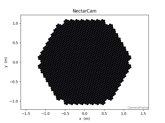
<ctapipe.visualization.mpl_camera.CameraDisplay object at 0x79f08b05d390>

You can also specify the initial image, cmap and norm (colomap and normalization, see below), title to use. You can specify ax if you want to draw the camera on an existing matplotlib Axes object (otherwise one is created).

To change other options, or to change options dynamically, you can call the relevant functions of the CameraDisplay object that is returned. For example to add a color bar, call add_colorbar(), or to change the color scale, modify the cmap or norm properties directly.

Choosing a coordinate frame

The CameraGeometry object contains a ctapipe.coordinates.Frame used by CameraDisplay to draw the camera in the correct orientation and distance units. The default frame is the CameraFrame, which will display the camera in units of meters and with an orientation that the top of the camera (when parked) is aligned to the X-axis. To show the camera in another orientation, it’s useful to apply a coordinate transform to the CameraGeometry before passing it to the CameraDisplay. The following Frames are supported:

• CameraFrame: The frame used by SimTelArray, with the top of the camera on the x-axis

• EngineeringCameraFrame: similar to CameraFrame, but with the top of the camera aligned to the Y axis

• TelescopeFrame: In degrees (on the sky) coordinates relative to the telescope Alt/Az pointing position, with the Alt axis pointing upward.

Note the the name of the Frame appears in the lower-right corner

fig, ax = plt.subplots(1, 3, figsize=(15, 4))
CameraDisplay(geom, image=image, ax=ax[0])
CameraDisplay(geom.transform_to(EngineeringCameraFrame()), image=image, ax=ax[1])
CameraDisplay(geom.transform_to(TelescopeFrame()), image=image, ax=ax[2])

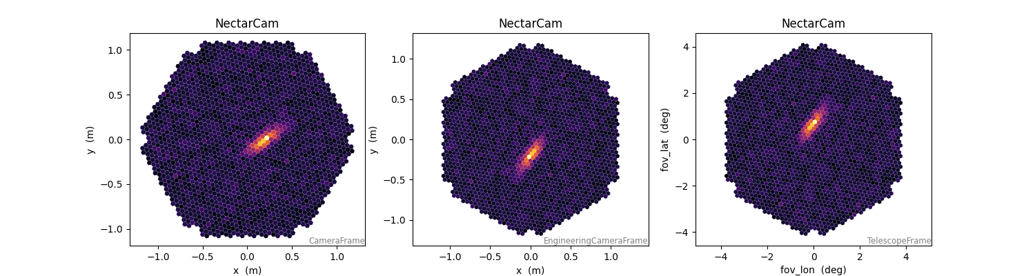
<ctapipe.visualization.mpl_camera.CameraDisplay object at 0x79f096d89390>

For the rest of this demo, let’s use the TelescopeFrame

geom_camframe = geom
geom = geom_camframe.transform_to(EngineeringCameraFrame())

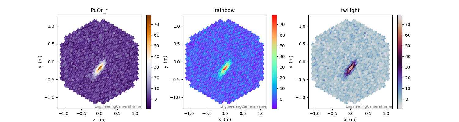
Changing the color map and scale

CameraDisplay supports any matplotlib color map It is highly recommended to use a perceptually uniform map, unless you have a good reason not to.

fig, ax = plt.subplots(1, 3, figsize=(15, 4))
for ii, cmap in enumerate(["PuOr_r", "rainbow", "twilight"]):
    disp = CameraDisplay(geom, image=image, ax=ax[ii], title=cmap)
    disp.add_colorbar()
    disp.cmap = cmap

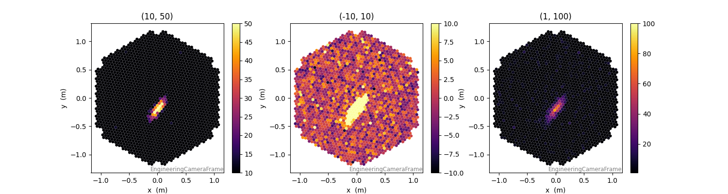
By default the minimum and maximum of the color bar are set automatically by the data in the image. To choose fixed limits, use:`

fig, ax = plt.subplots(1, 3, figsize=(15, 4))
for ii, minmax in enumerate([(10, 50), (-10, 10), (1, 100)]):
    disp = CameraDisplay(geom, image=image, ax=ax[ii], title=minmax)
    disp.add_colorbar()
    disp.set_limits_minmax(minmax[0], minmax[1])

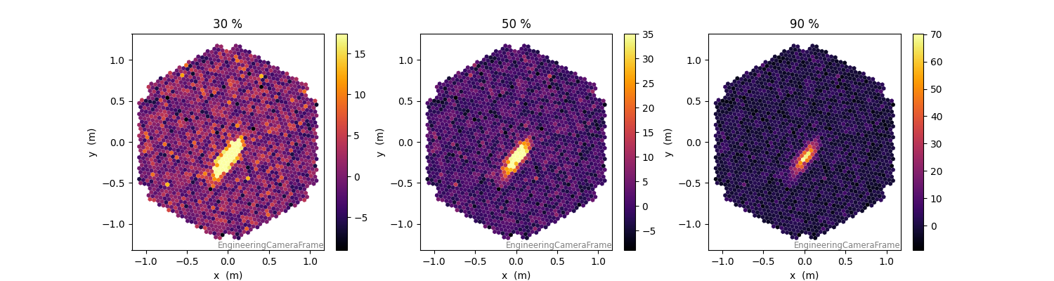
Or you can set the maximum limit by percentile of the charge distribution:

fig, ax = plt.subplots(1, 3, figsize=(15, 4))
for ii, pct in enumerate([30, 50, 90]):
    disp = CameraDisplay(geom, image=image, ax=ax[ii], title=f"{pct} %")
    disp.add_colorbar()
    disp.set_limits_percent(pct)

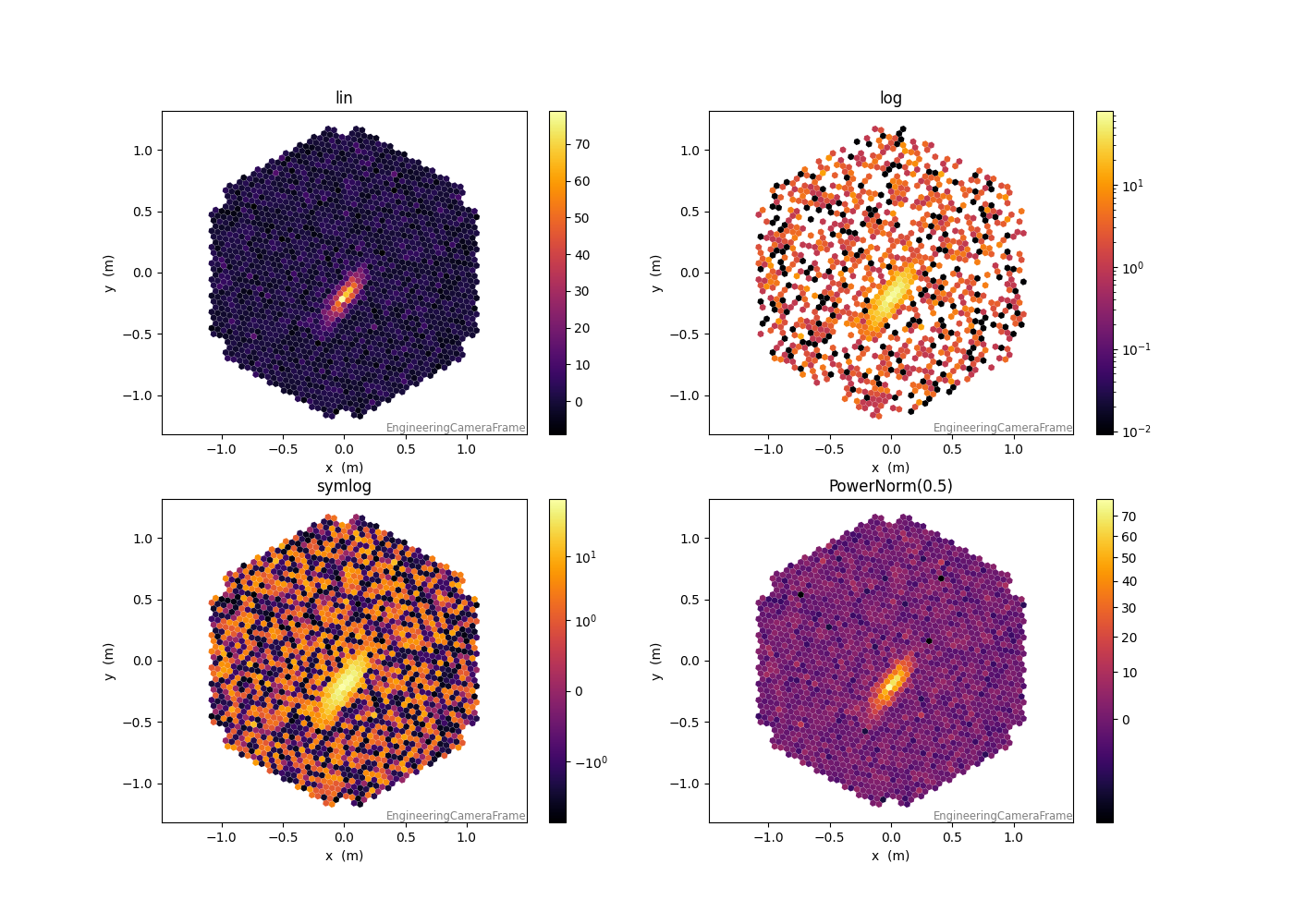
Using different normalizations

You can choose from several preset normalizations (lin, log, symlog) and also provide a custom normalization, for example a PowerNorm:

fig, axes = plt.subplots(2, 2, figsize=(14, 10))
norms = ["lin", "log", "symlog", PowerNorm(0.5)]

for norm, ax in zip(norms, axes.flatten()):
    disp = CameraDisplay(geom, image=image, ax=ax)
    disp.norm = norm
    disp.add_colorbar()
    ax.set_title(str(norm))

axes[1, 1].set_title("PowerNorm(0.5)")
plt.show()

Overlays

Marking pixels

here we will mark pixels in the image mask. That will change their outline color

fig, ax = plt.subplots(1, 2, figsize=(10, 4))
disp = CameraDisplay(
    geom, image=image, cmap="gray", ax=ax[0], title="Image mask in green"
)
disp.highlight_pixels(mask, alpha=0.8, linewidth=2, color="green")

disp = CameraDisplay(
    geom, image=image, cmap="gray", ax=ax[1], title="Image mask in green (zoom)"
)
disp.highlight_pixels(mask, alpha=1, linewidth=3, color="green")

ax[1].set_ylim(-0.5, 0.5)
ax[1].set_xlim(-0.5, 0.5)

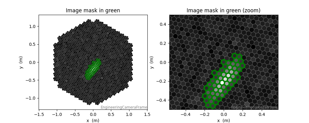
(-0.5, 0.5)

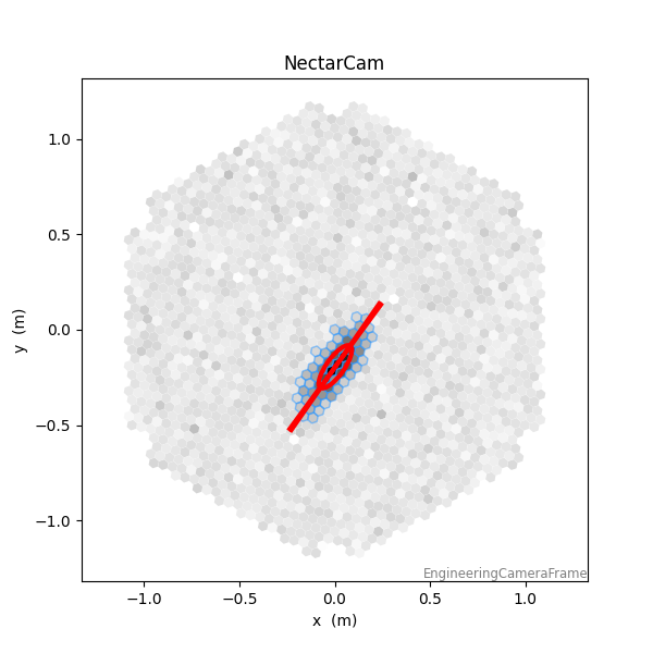
Drawing a Hillas-parameter ellipse

For this, we will first compute some Hillas Parameters in the current frame:

clean_image = image.copy()
clean_image[~mask] = 0
hillas = hillas_parameters(geom, clean_image)

plt.figure(figsize=(6, 6))
disp = CameraDisplay(geom, image=image, cmap="gray_r")
disp.highlight_pixels(mask, alpha=0.5, color="dodgerblue")
disp.overlay_moments(hillas, color="red", linewidth=3, with_label=False)

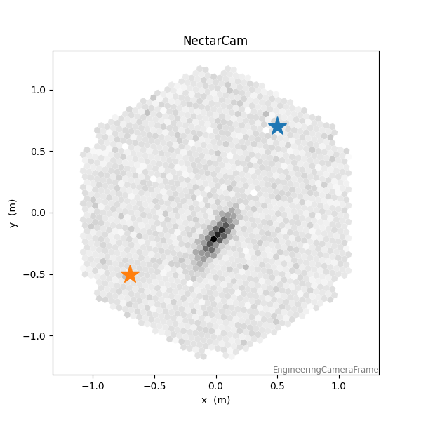
Drawing a marker at a coordinate

This depends on the coordinate frame of the CameraGeometry. Here we will specify the coordinate the EngineerngCameraFrame, but if you have enough information to do the coordinate transform, you could use ICRS coordinates and overlay star positions. CameraDisplay will convert the coordinate you pass in to the Frame of the display automatically (if sufficient frame attributes are set).

Note that the parameter keep_old is False by default, meaning adding a new point will clear the previous ones (useful for animations, but perhaps unexpected for a static plot). Set it to True to plot multiple markers.

plt.figure(figsize=(6, 6))
disp = CameraDisplay(geom, image=image, cmap="gray_r")

coord = c.SkyCoord(x=0.5 * u.m, y=0.7 * u.m, frame=geom.frame)
coord_in_another_frame = c.SkyCoord(x=0.5 * u.m, y=0.7 * u.m, frame=CameraFrame())
disp.overlay_coordinate(coord, markersize=20, marker="*")
disp.overlay_coordinate(
    coord_in_another_frame, markersize=20, marker="*", keep_old=True
)

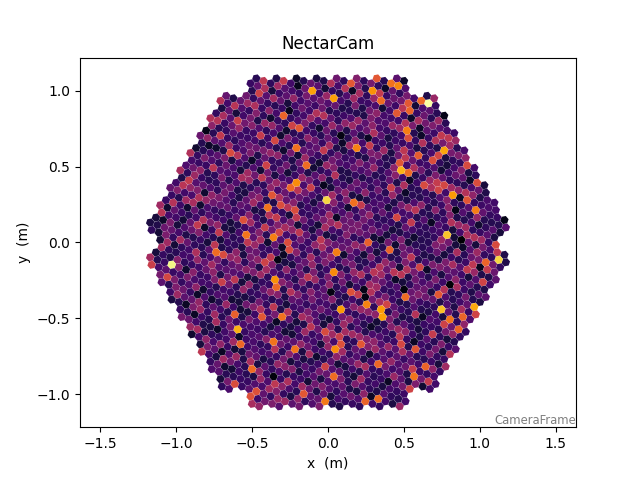
Generating an animation

Here we will make an animation of fake events by re-using a single display (much faster than generating a new one each time)

subarray = SubarrayDescription.read("dataset://gamma_prod5.simtel.zst")
geom = subarray.tel[1].camera.geometry

fov = 1.0
maxwid = 0.05
maxlen = 0.1

fig, ax = plt.subplots(1, 1, figsize=(8, 6))
disp = CameraDisplay(geom, ax=ax)  # we only need one display (it can be re-used)
disp.cmap = "inferno"
disp.add_colorbar(ax=ax)


def update(frame):
    """this function will be called for each frame of the animation"""
    x, y = np.random.uniform(-fov, fov, size=2)
    width = np.random.uniform(0.01, maxwid)
    length = np.random.uniform(width, maxlen)
    angle = np.random.uniform(0, 180)
    intens = width * length * (5e4 + 1e5 * np.random.exponential(2))

    model = toymodel.Gaussian(
        x=x * u.m,
        y=y * u.m,
        width=width * u.m,
        length=length * u.m,
        psi=angle * u.deg,
    )
    image, _, _ = model.generate_image(
        geom,
        intensity=intens,
        nsb_level_pe=5,
    )
    disp.image = image


# Create the animation and convert to a displayable video:
anim = FuncAnimation(fig, func=update, frames=10, interval=200)
plt.show()

Once Loop Reflect

Using CameraDisplays interactively

CameraDisplays can be used interactively when displayed in a window, and also when using Jupyter notebooks/lab with appropriate backends.

When this is the case, the same CameraDisplay object can be re-used. We can’t show this here in the documentation, but creating an animation when in a matplotlib window is quite easy! Try this in an interactive ipython session:

Running interactive displays in a matplotlib window

ipython -i –maplotlib=auto

That will open an ipython session with matplotlib graphics in a separate thread, meaning that you can type code and interact with plots simultaneneously.

In the ipython session try running the following code and you will see an animation (here in the documentation, it will of course be static)

First we load some real data so we have a nice image to view:

DATA = "dataset://gamma_20deg_0deg_run1___cta-prod5-lapalma_desert-2158m-LaPalma-dark_100evts.simtel.zst"

with EventSource(
    DATA,
    max_events=1,
    focal_length_choice="EQUIVALENT",
) as source:
    event = next(iter(source))

tel_id = list(event.r0.tel.keys())[0]
geom = source.subarray.tel[tel_id].camera.geometry
waveform = event.r0.tel[tel_id].waveform
n_chan, n_pix, n_samp = waveform.shape

Running the following the will bring up a window and animate the shower image as a function of time.

disp = CameraDisplay(geom)

for ii in range(n_samp):
    disp.image = waveform[0, :, ii]
    plt.pause(0.1)  # this lets matplotlib re-draw the scene

The output will be similar to the static animation created as follows:

fig, ax = plt.subplots(1, 1)
disp = CameraDisplay(geom, ax=ax)
disp.add_colorbar()
disp.autoscale = False


def draw_sample(frame):
    ax.set_title(f"sample: {frame}")
    disp.set_limits_minmax(200, 400)
    disp.image = waveform[0, :, frame]


anim = FuncAnimation(fig, func=draw_sample, frames=n_samp, interval=100)
plt.show()

Once Loop Reflect

Making it clickable

Also when running in a window, you can enable the disp.enable_pixel_picker() option. This will then allow the user to click a pixel and a function will run. By default the function simply prints the pixel and value to stdout, however you can override the function on_pixel_clicked(pix_id) to do anything you want by making a subclass

class MyCameraDisplay(CameraDisplay):
    def on_pixel_clicked(self, pix_id):
        print(f"{pix_id=} has value {self.image[pix_id]:.2f}")


disp = MyCameraDisplay(geom, image=image)
disp.enable_pixel_picker()

then, when a user clicks a pixel it would print:

pixel 5 has value 2.44